Multirate Sampling

A CBC signal spends most of its time at low frequency, where the bandwidth requirements are modest, then rapidly sweeps through high frequencies in the last fraction of a second. Representing the entire segment at the full 2048 Hz sample rate wastes memory and computation on the low-frequency inspiral. Dyadic multirate sampling assigns a different (lower) sample rate to each time interval, keeping the total number of samples small while preserving all information relevant to detection.

Initialising the sampler

TDMultirateSampler computes the bin boundaries analytically from the prior mass range and the signal model:

from sage.dsp.multirate_sampling import TDMultirateSampler

mrs = TDMultirateSampler(
    prior_low_mass=7.0,      # minimum component mass in the prior (solar masses)
    prior_high_mass=50.0,    # maximum component mass in the prior (solar masses)
    signal_low_freq_cutoff=20.0,   # Hz — lowest frequency in the waveform
    sample_rate=2048,              # Hz — native sample rate of the whitened data
    signal_length=12.0,            # seconds — total segment length
    lowest_allowed_fs=64.0,        # Hz — minimum sample rate for any bin
    tc_inject_lower=11.0,          # seconds — earliest possible coalescence time
    tc_inject_upper=11.2,          # seconds — latest possible coalescence time
    safe_nyquist_gap=0.0,
)

How the bins work

TDMultirateSampler builds a set of time–frequency bins, each covering a contiguous time interval of the segment and assigned a specific sample rate. The merger-containing region is kept at the full 2048 Hz; earlier portions are progressively downsampled.

Inspect the bins:

for start, end, fs in mrs.detailed_bins:
    print(f"  [{start/2048.:6.3f} s, {end/2048.:6.3f} s]  →  {fs} Hz")

[  0.000 s,  9.018 s]  →  128 Hz
[  9.018 s, 10.667 s]  →  256 Hz
[ 10.667 s, 10.938 s]  →  512 Hz
[ 10.938 s, 11.353 s]  → 2048 Hz
[ 11.353 s, 12.000 s]  →   64 Hz

final_eff_duration = sum(
    int((end - start) / (2048 / fs))
    for start, end, fs in mrs.detailed_bins
)
print(f"Total samples after compression: {final_eff_duration}")
print(f"Equivalent duration at 2048 Hz:  {final_eff_duration / 2048.:.3f} s")
# Total samples after compression: 2605
# Equivalent duration at 2048 Hz:  1.272 s

The post-merger region (after the latest possible tc) is assigned the lowest sample rate (64 Hz) because there is no signal power there — only noise. This brings the compressed representation down to roughly 2600 samples from the original 24 576.

Visualise the time–frequency tiling:

mrs.plot_multirate_tf()

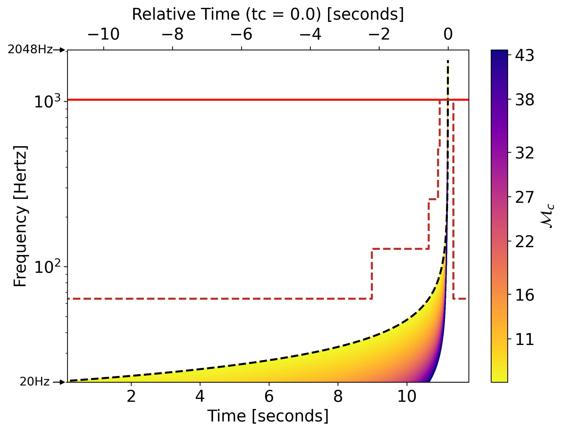
Frequency vs time curves of GWs generated from the testing dataset parameter distributions, coloured by chirp mass. The dashed black line shows the frequency profile of a GW with the lowest possible chirp mass (longest duration). The solid red line shows the Nyquist limit at 1024 Hz given a sample rate of 2048 Hz; the dashed red line shows the modified Nyquist limit after applying the multi-rate sampling algorithm.

Applying multirate sampling

TorchMultiRateSampler performs the actual downsampling in a torch.compile-compatible manner:

import numpy as np
from sage.dsp.multirate_sampling import TorchMultiRateSampler

compress = TorchMultiRateSampler(
    bins=mrs.detailed_bins,
    original_fs=data_cfg.sample_rate,
    min_fs=int(np.min(mrs.detailed_bins[:, 2])),
)

The forward method takes a real time-domain tensor (B, n_det, T) and returns the compressed representation of the same shape prefix but with the time axis shortened:

out = compress.forward(whitened)
# whitened:  (B, n_det, 24576)  →  out: (B, n_det, 2605)

Applying to the whitened noisy signal

compressed_noisy = compress.forward(whitened)

fig, axes = plt.subplots(2, 1, figsize=(12, 6), sharex=False)
axes[0].plot(whitened[0][0].detach().cpu().numpy())
axes[0].set_title("Whitened noisy signal (24 576 samples)")
axes[1].plot(compressed_noisy[0][0].detach().cpu().numpy())
axes[1].set_title("After multirate compression (2 605 samples)")
plt.tight_layout()

The compressed trace preserves the merger region at full resolution while the long low-frequency inspiral is represented by far fewer samples.

Applying to pure signal

import torch

# Convert FD signal batch to TD first
signal_td = torch.fft.irfft(signal_batch, dim=-1)
compressed_signal = compress.forward(signal_td)

fig, axes = plt.subplots(2, 1, figsize=(12, 6))
axes[0].plot(signal_td[0][0].detach().cpu().numpy())
axes[0].set_title("Raw signal (time domain)")
axes[1].plot(compressed_signal[0][0].detach().cpu().numpy())
axes[1].set_title("Multirate-compressed signal")
plt.tight_layout()

On pure signal the chirp structure is still clearly visible in the merger bin, while the long low-amplitude inspiral is compressed to a handful of samples.

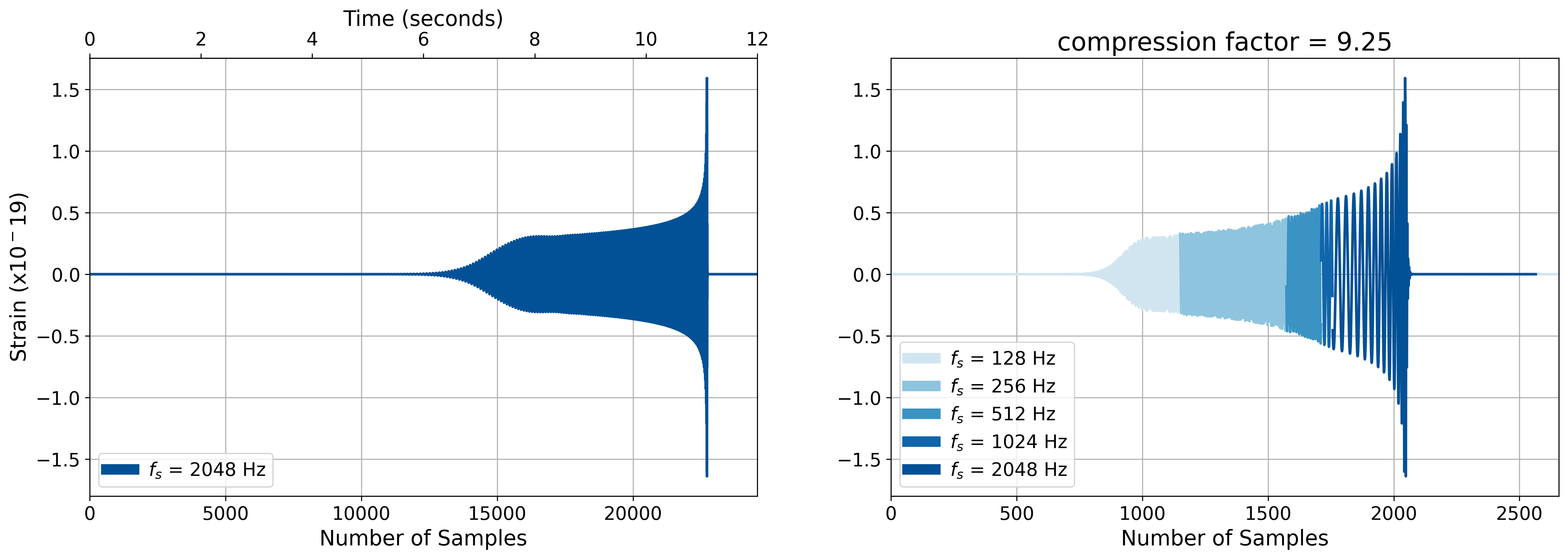
Example application of multirate sampling on a BBH template with \(m_1 = 20\,M_\odot\), \(m_2 = 10\,M_\odot\), zero spins, and \(t_c = 11.1\,\mathrm{s}\). Colours indicate the effective sampling frequency \(f_s\) of each section of the compressed signal; \(f_s = 2048\,\mathrm{Hz}\) corresponds to an unaltered (full-rate) section.