Overview
Sage is an end-to-end supervised learning pipeline that tackles gravitational-wave CBC
detection by systematically identifying and mitigating 11 interconnected learning biases.
All modules are optimised for CPU and GPU (torch.compile-compatible) usage.
How to use this guide
The User Guide sidebar entries are arranged in the exact order you should follow them — start at the top and work your way down. Each page builds on the one before it, so following them in sequence is the smoothest path from a fresh install to a fully-trained Sage model. You do not need to read everything in one sitting; every page is self-contained enough that you can pick up exactly where you left off.
Tip
Don’t be put off by the number of steps — each one is short and focused on a single concept. Work through them at your own pace and you will have a complete picture of the pipeline before you know it. You’ve got this!
The diagram below shows the full Sage methodology at a glance, so you can always orient yourself within the bigger picture as you work through the guide.
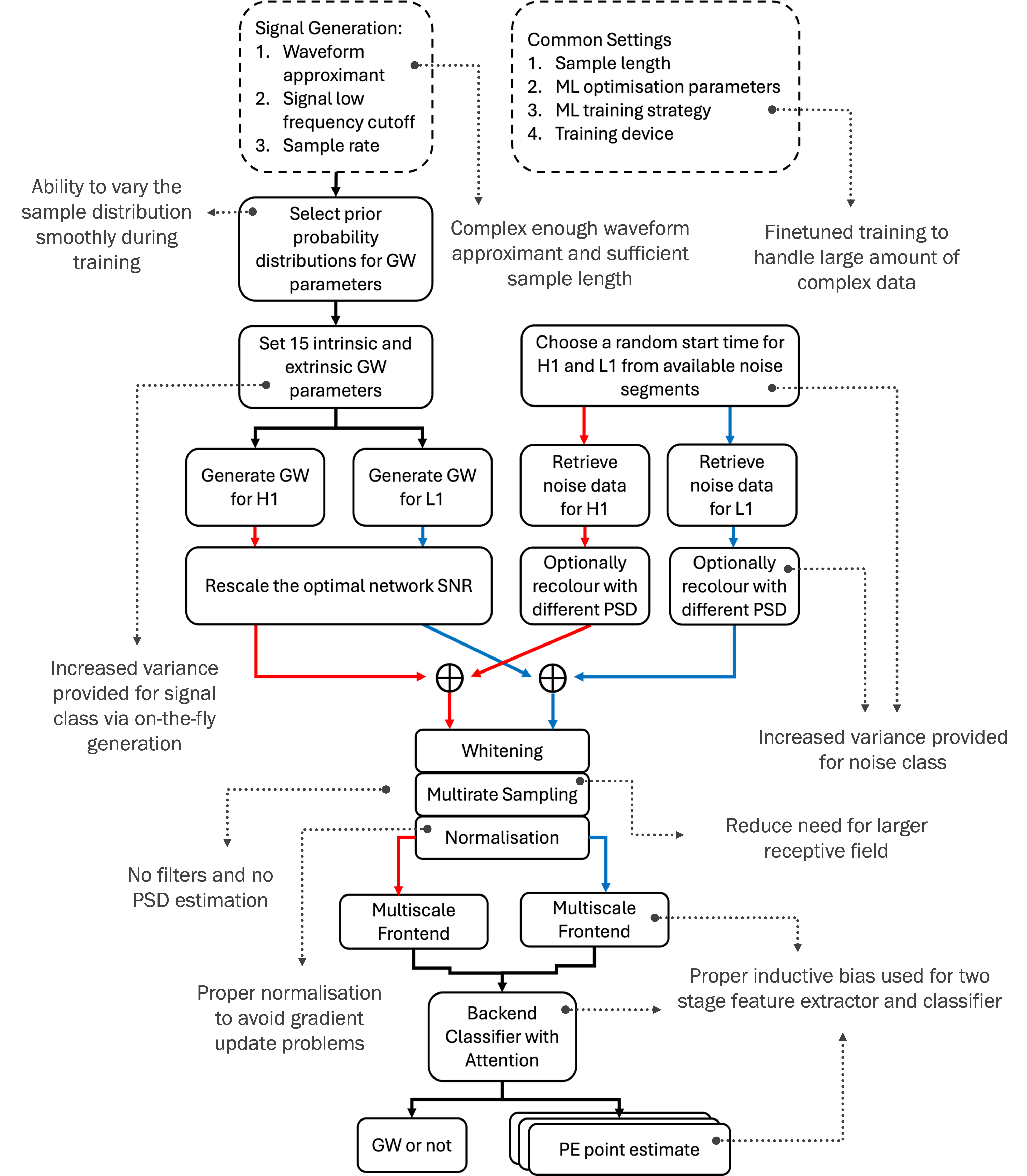
The complete Sage pipeline — from raw GWOSC strain data through signal processing, on-the-fly data generation, and neural-network training, to final evaluation.
Modules
Module |
Description |
|---|---|
Network components: frontend CNN, backend ResNet-CBAM, loss functions |
|
Configuration management, logging, constants, interpolation, math utilities |
|
Waveform generation, noise sampling, PSD handling, data primitives |
|
Digital signal processing: FFT, whitening, multirate sampling, Welch PSD |
|
Execution orchestration: |
|
Training/validation loops, callbacks, schedulers, compile manager |
|
Diagnostic plots: ROC curves, efficiency, parameter recovery, loss curves |
|
Legacy run configs and shared data configs (see |
|
Checkpointing, timing utilities, Condor job submission |
Architecture
Sage uses a two-stage neural network:
Frontend — per-detector multi-scale 1D CNN (
ConvBlock) that extracts temporal features across a wide range of time scales using five parallel convolutions at different kernel sizes.Backend — 2D ResNet with CBAM (Convolutional Block Attention Module) attention (
ResNet) that processes the stacked per-detector feature maps and produces a compact feature vector.
The network head outputs:
A ranking statistic (raw logit for BCE classification).
Heteroscedastic point estimates (mean + log-variance) for each regression target (e.g. chirp mass, coalescence time).
Training pipeline
Training is performed on-the-fly (OTF) — no fixed dataset is pre-generated. At each iteration:
Gravitational-wave signals are sampled from the prior (
DistributionSampler), projected onto detectors, and SNR-rescaled.Real LIGO noise windows are asynchronously fetched from a memory-mapped file (
MemmapNoiseSampler).Signals are injected at random positions in the noise batch.
The pipeline applies FD whitening (
FiducialWhitening) and dyadic multirate sampling (MultirateSampler).The loss is computed using
BCEWithPEsigmaLoss— BCE classification combined with heteroscedastic regression and coupling regularisation for simultaneous detection and parameter estimation.
Waveform generation
Two GPU-native batched approximants are provided:
IMRPhenomD— aligned-spin frequency-domain waveforms,torch.compile-compatible (GRAPH_READY = True).IMRPhenomPv2— precessing-spin extension via the PhenomPv2 “twist-up” formalism.
Waveform parameters are drawn from a YAML-configured prior using
DistributionSampler.
Signal processing
The DSP stack (sage.dsp) includes:
Whitening — frequency-domain whitening with inverse spectrum truncation.
Multirate sampling — dyadic time-domain downsampling to focus resolution around the merger.
FD multibanding — frequency-domain multirate representation for compute-efficient signal coverage.
Prior-median heterodyning — carrier-frequency removal that collapses the CBC chirp to a narrow band, reducing required sample rates.
Noise handling
Real strain noise — GWOSC O3a/O3b data accessed via memory-mapped files.
Coloured / recoloured noise — synthetic noise coloured to a target PSD.
Glitch oversampling — GW Classify-labelled glitch segments are oversampled to expose the network to realistic transient artefacts.